To tree or not to tree: an introduction of phylogenetic networks

Phylogenetic reconstruction is of crucial importance to elucidate bacterial population structure, epidemiology and evolutionary histories. By far phylogenetic networks and trees are the most common approaches used for studying the evolutionary history of a bacterial population. However, concepts and methodology underlying phylogenetic reconstruction can be challenging to beginners. As such, I share my notes on relevant literature in this post to address these obstacles. In particular, I compare different kinds of phylogenetic networks to show their pros and cons under various conditions.

1. Definitions

Phylogenetic network: any network in which nodes represent taxa and edges represent evolutionary relationships between taxa¹. Huson and Bryant listed the following three kinds of phylogenetic networks.

• Phylogenetic trees: a rooted or unrooted leaf-labelled tree that represents the evolutionary history of a set of taxa, possibly with branch lengths¹. As I have explained in an earlier post, the tree only relies on evolutionary models of nucleotide substitutions. For instance, maximum-likelihood (ML) models consist of assumptions for base frequencies and rate variation across sites. Further, Huson and Bryant point out that no tree-based model can accurately takes reticulate evolutionary events into account¹.
• Split network: represents incompatibilities and uncertainty within and between data sets¹. In such a network, parallel edges are used to represent splits and their weights computed from genomic data¹ (Fig. 1). The network provides an “implicit” representation of an evolutionary history because the network may contain nodes that do not represent ancestral taxa¹, which differs from both phylogenetic trees and reticulate networks. It has been shown that split networks can extract phylogenetic signals that are not captured by phylogenetic trees¹.
  • Split: a partition (cut, division) of taxa into two nonempty subsets of data¹. In every split network, each edge is associated with a split of taxa, yet there may be a number of parallel edges associated with the same split¹(Fig. 2). Deletion of all edges associated with the same split cuts the original network into precisely two disconnected components corresponding to two subsets of the taxa¹.
    • Trivial splits¹: edges ended at tips (terminal edges). The number of trivial edges equals that of taxa.
    • Principal splits: I call internal edges (non-terminal edges) principal splits. Evidently, the number of principal splits is the count of sets of parallel edges.
    • Compatible set of splits (phylogenetic tree) and incompatible set of splits (phylogenetic network)³.
  • Edge length: every split network is a weighted network, where the edge length is proportional to the weight of the associated split¹.
  • Edge directionality: most split networks published to date are unrooted¹. As such, the edges are undirected in these networks.
  • Equivalent representation: a table of splits (binary entries) and weights (Fig. 2b).
• Reticulate network: “explicitly” represents evolutionary histories in the presence of reticulate events, including hybridisation, horizontal gene transfer (HGT) and recombination, and is generally shown as a phylogenetic tree with additional edges¹. In the network, internal nodes correspond to hypothetical ancestors, edges represent patterns of descent, and every node having more than two parents indicates reticulate events such as recombination and HGT¹ (Fig. 1). The network is usually rooted and hence has directed edges¹.

Figure 1. Split network (a) versus reticulate network (b) of the same set of taxa. See the caption of Fig. 3. in the article by Huson and Bryant for details¹.

Figure 2. Edges and taxa subsets corresponding to subdivisions in a split network. Parallel edges denote splits associated with the same split. These edges have to be parallel, otherwise, the removal of these edges cannot split the network into two disconnected components. One side of taxa subsets and edges representing Split 10 are highlighted with boldface. Notably, the table or network does not necessarily exhaust all possible splits of the taxa. See the caption of Fig. 4. in the article by Huson and Bryant for more details.

Figure 3. Every split network represents a unique collection of splits, but the same collection of underlying splits does not result in a unique split network¹. There are three principal splits of these six taxa since there are three sets of parallel edges. See the caption of Fig. 5. in the article by Huson and Bryant for details.

2. Utility and interpretations

2.1. Split networks

Huson and Bryant suggest to use split networks for inspecting the relatedness between taxa and evaluating the reliability of reconstructed phylogenetic trees¹. Accordingly, the split network provides us with a sensible starting point for phylogenetic inference.

• A summary network deduced from multiple trees¹, because the topology of every phylogenetic tree indicates a collection of taxa splits. A particular type of summary networks is the consensus network.
  • Consensus network: a summary set of splits that code each tree as a set of splits and it is recommended to incorporate p-values into the network, namely, to assign a confidence interval (CI) to each split¹. Any phylogenetic tree resulting from a zero-containing CI has weight zero and is believed to be absent in the space of plausible trees (See Fig. 6 in the article by Huson and Bryant). We say the split network does not contain a tree in this situation¹.

2.2. Reticulate networks

• Hybridisation network¹.
• Ancestor recombination graph or recombination network¹.

3. Methods and software for constructing split networks

• Model-based methods¹, including split decomposition².
• SplitTree4: implements many published methods for inferring split trees, including median networks, parsimony splits, split decomposition, consensus networks, etc., as well as methods for constructing reticulate networks, including recombination networks and hybridisation networks¹. It also provides a graphical front-end for ML analysis using PhyML and parsimony analysis using PHYLIP.

3.1. Neighbor-Net method

Notes in this section are based on citation 3. Please see the original article for details of the Neighbor-Net method.

• A distance based method (with a distance matrix) inspired by the neighbour-joining (NJ) method. In SplitTree4, the uncorrected P distance (that is, the percentage of SNPs in an alignment of two sequences) is used.
• Major steps: (1) construct a collection of weighted splits, (2) represent these splits using a split network, also known as a splits graph.
  • Every splits graph is a graphical representation of a collection of weighted splits identified using the iterative agglomeration process.
  • A collection of compatible splits forms a tree.
  • A collection of incompatible splits is represented by a network with cycles or boxes. Each group of parallel edges represent the same split.
  • Branch or edge length: weight of the corresponding split.
  • The graph may be three-dimensional, but can be equivalently represented by a planar network.
  • The split graph is not necessarily unique, hence only displays conflicting signals rather than explicit evolutionary history of which reticulation took place. The reticulations can be located using a splits graph, but should be validated using other techniques.
• Advantage: higher resolution than split decomposition.
• Iterative agglomeration process, which guarantees statistical consistency of the Neighbor-Net method.
  • Initiation: no neighbourhood of nodes is assigned.
  • Formulae used for iteratively selecting pairs of nodes for agglomeration.
    • Starting from single-element clusters, the Neighbor-Net algorithm agglomerates taxa into clusters (namely, form new nodes).
    • The distance between two clusters is the average distance between elements in each cluster.
    • Selection of neighbouring nodes for minimising the distance between two clusters (standard NJ formula).
    • Software implementing the Neighbor-Net algorithm keeps a list of agglomerations, everyone of which replaces three nodes with two.
  • Formula used for reducing the distance matrix after each agglomeration of nodes.
    • Reason: nodes become fewer after every round of agglomeration.
    • Recalculate distances after every round of agglomeration.
  • Estimating the weight of each split using a least-squares framework as the NJ algorithm.
    • The phyletic distance between two taxa equals the sum of weights of splits separating them, or the length of a shortest path connecting them.
    • The Standard topological matrix of a tree is a three-dimensional binary matrix.
      • Each row represents a combination of two taxa.
      • Each column represents a split, trivial or principal.
      • A full-rank matrix.
    • Weighted least squares (WLS) estimates of split weights (a column vector) are computed from the standard topological matrix and the vectorised distance matrix.
  • Outcome: a (conceptual) circular collection of splits. Taxa are placed on this circle and each split is given y cutting the circle along a line, always resulting in a planar graph.

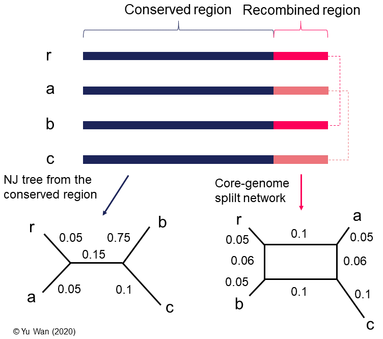
Figure 4. A comparison between an NJ tree and a split network based on the same core-genome alignment. Three bacterial genomes (a, b, and c) are aligned to their reference genome r, and their core-genome (arbitrarily defined as sites present in all genomes). The core-genome is comprised of a conserved part and a recombined region, which is assumed to have an equal length for simplicity. Assume the split network is constructed from uncorrected P distances using the Neighbor-Net method. The conserved part between genomes is coloured in dark blue, while two kinds of shared recombination regions are coloured in bright pink and light pink, respectively. For simplicity, I assume there is no divergence between copies of the same recombined region. As a result, owing to the identity of recombined regions in the core-genome, the proximity between a, b, c, and r in the split network differs from that in the NJ tree, which only accounts for the conserved region. The phyletic distance between two taxa can be calculated from the shortest path connecting them. For instance, d(r, c) = 0.05 + 0.1 + 0.06 + 0.1 = 0.31. Note that a phylogenetic tree that is compatible to all phyletic distances in the split network does not exist, justifying the necessity of using a split network to represent the relationship between the taxa.

---

## References

1. Huson, D. H. & Bryant, D. Application of Phylogenetic Networks in Evolutionary Studies. Mol. Biol. Evol. 23, 254–267 (2005). This is a comprehensive review of phylogenetic networks and relevant statistical tests.
2. Bandelt, H.-J. & Dress, A. W. M. A canonical decomposition theory for metrics on a finite set. Adv. Math. (N. Y). 92, 47–105 (1992).
3. Bryant, D., & Moulton, V. (2004). Neighbor-Net: An Agglomerative Method for the Construction of Phylogenetic Networks. Molecular Biology and Evolution, 21(2), 255–265. https://doi.org/10.1093/molbev/msh018.